Some of the spreadsheets that we encounter contain large data sets that may be difficult to analyze. Google Sheets has a feature called conditional formatting that can make things easier for you.

What is conditional formatting

Conditional formatting lets you automatically modify or format your data according to the rules you set. This makes it easier for you to analyze your data and see significant patterns or trends. You can use conditional formatting to a range of cells and apply different formatting styles such as highlighting cells and changing the font color, size, and style.

When to use conditional formatting

Conditional formatting can be used when you want to visualize the data in your spreadsheet, compare values, see patterns and trends, differentiate, and emphasize specific cells.

For instance, you can use conditional formatting to check if your actual spending exceeded the budget you set. If you’re a student, you can use this to determine if your grades are good or not. There is a wide range of applications where you can use conditional formatting.

Types of conditional use formatting

The conditional formatting you can do in Google Sheets are:

• Bold, italicize, underline, and strikethrough cell values

• Change font color

• Change background color

• Apply a color scale to the data

There are also several types of formatting rules that you can apply to texts, numbers, or dates. 

Formatting texts

You can use the formatting styles to cells if:

• Cell is empty

• Cell is not empty

• Text contains

• Text does not contain

• Text starts with

• Text ends with

• Text is exact

Formatting numbers

The following formatting rules can be applied to the numbers in your spreadsheet.

• Greater than 

• Greater than or equal to

• Less than

• Less than or equal to

• Is not equal to

• Is between

• Is not between

Formatting dates

You can also use conditional formatting for the dates in your spreadsheet. These are the rules that you can apply:

• Date is

• Date is before

• Date is after

How to use conditional formatting

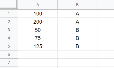
Let’s take an example to demonstrate how conditional formatting works. In the sample data below, we will format the cells in column A with values greater than 100.

1. Highlight the data in column A, cells A1 to A5.

2. Go to the toolbar and click on Format > Conditional Formatting.

2. A box will appear on the right side of your screen containing the options for conditional formatting.

3. In the drop-down option under the “Format rules”, click “Greater Than”, and type “100” as the value.

We will use the default formatting style, but you can modify the style according to your preference.

4. Click “Done”.

You will see that the values in column A that are greater than 100 are highlighted based on the formatting style that we set.

Conditional formatting based on another cell

Now that you’ve learned the basics of conditional formatting, let’s move on to a more complicated example.

You can also use conditional formatting based on another cell. This means that you will apply the format style to a specific cell/s with reference to the value of other cell/s. To illustrate this, we will use the previous example.

We will highlight the cells in column B if their corresponding value in column A is greater than or equal to 100. To do this,

1. Highlight the data under column B, cells B1 to B5.

2. Click on Format > Conditional Formatting.

3. In the conditional formatting options, select “Custom format is” under the “Format rules” drop-down.

4. For the value, type the following formula:

= A1 > = 100

Let’s break down the formula.

• = (equal sign) indicates that you are writing a formula.

• A1 tells us that the formula will apply starting from cell A1 down to the next cells.

• > = 100 means that the format will apply to cells whose corresponding values are greater than or equal to 100.

5. Click “Done”.

You’ll see that even if we typed column A in the custom formula, the cells in column B were the ones highlighted.

More complex conditional formatting

The examples we have provided here are just a small taste of what conditional formatting can do. You can set more than one parameter and have plenty of conditional formatting formulas running on a sheet to make your data significantly easier to read.

The custom formulas we briefly touched on in the above section can become quite complex and can be great for working with others by importing locked data from other sheets or simply for the use of making it easier to see data at a glance for your coworkers.

Copying conditional formatting

Let’s say you like the conditional formatting that you’ve seen on another sheet. You can easily copy that formatting into a new sheet. This can also be handy if you’re working with new sheets frequently and don’t have to have to set up the exact same conditional formatting every time.

One of the simplest ways to copy over conditional formatting is to use the Paste Special command. To use this method, you just have to follow these steps,

1. Select the range of cells that you want to copy the conditional formatting from

2. Use the Ctrl + C keyboard shortcut to copy (or right-click and select copy)

3. Select the new range of cells that you want the conditional formatting copied to

4. Right-click on the new selected cells

5. Navigate to Paste special>Paste format only (you could also use the keyboard shortcut that is Ctrl+Alt+V)

6. If you need to repeat this process for more rows or columns you can just repeat steps 3-5. You don’t have to select the cells again.

When you copy over the conditional formatting in this way in the same sheet, it doesn’t create a new rule but instead forces the existing formatting to include the new ranges.

Conclusion

Applying conditional formatting to your spreadsheet allows you to save time in analyzing the data. By creating custom formatting styles, you can easily see patterns and differentiate the data in your spreadsheet.